|
|||||||
|
| Throwing dice
When an ordinary six-sided die is thrown, we cannot predict the outcome. Hence a die is often used in games to give a number selected at random from the range 1 to 6. A single number by itself cannot be random. If you throw a die and you get a 3, there is nothing random about the 3 on its own. The randomness stems from the fact that you could just have easily had a 1, 2, 4, 5 or 6. The effect of the die is to select a number from this range. It is the selection that is random, not the result, but we often use the term ‘random number’ to describe numbers that have been selected at random from a range of possibilities. 1. Throw a six-sided die 50 times and count the how often each number comes up. We expect to get numbers 1, 2, 3, 4, 5 or 6 with equal probability. Thus each number should come up about equally often. |
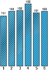
Below we see the results of 1,000 throws of a six-sided die. We see that the number 4 occurs most often. Does this mean that the die is not fair? Perhaps with another 1000 throws the results would even out! Such important questions are the business of statistics.
|
| Distributions
2. Throw two six-sided dice at the same time and add the numbers obtained. The result will be a number between 2 and 12. Do this 50 times and count the how often each result occurs. Do some numbers come up more often than others?
|
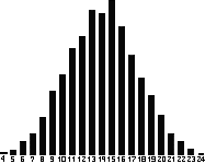
The diagram (left) shows the result of throwing two dice 1,000 times. 3. What do you suppose will happen if three or four dice are thrown at the same time, and their numbers added? Try it and see. The result shown right was obtained by throwing four dice 5,000 times. As the number of dice increases, the distribution of results approaches the bell-shaped normal or Gaussian distribution. Many natural phenomena also approximate this distribution, for example the distribution of people’s height around the average. |
| Random numbers
The behaviour of computers is determined by a program and totally predictable. So how can they generate can generate random numbers? Suppose we want a number that is randomly selected from the range of integers 1 to 6, each number occurring with equal probability, but with no predictable pattern. A computer would do something like the following: We use the notation x mod y to denote the remainder when x is divided by y. Start with any initial integer S0 (called the seed). Suppose we set S0 = 12,345. Let Ri denote the ith random number. To generate Rn, perform these calculations: Sn = (Sn–1 The large numbers are chosen to prevent a repeating pattern.
|
4. (Harder, optional) Use a calculator to complete the following table of numbers generated by this method. [You will need a 10 digit calculator. First try a simple example: e.g. 20 mod 6. You will need to determine how many times 6 divides 20 (an integer).]
The numbers are not random, but they satisfy most statistical tests for randomness. Each number comes up equally often, and there is no obvious relationship between one number and the next. Numbers of this kind are sometimes called pseudo-random. |
||||||
|
'Random' fractals
|
|
|
Random numbers can be used to generate totally predictable fractals! |
|
|
5. Mark vertices of |
|
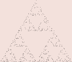
| Gradually a Sierpinski sieve appears, with vertices at A, B and C. The more points drawn, the clearer the sieve will be. The figure shows the effect after 500, 5,000 and 50,000 points have been plotted.
This is a random IFS method for generating the sieve. It uses three rules. The rule for A is |
 |
|
6. Show that, with coordinates (0,0), (1,0) and (0.5,1) for A, B and C, the above equations give the mappings used for the sieve in the program of Section 10. |
|
| A fractal fern (I)
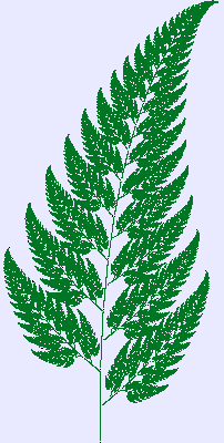
The rules used in an IFS can be more complicated than those we have used so far. Suppose we use the following four rules: Rule 1: x' = 0 Rule 2: x' = 0.85x + 0.04y Rule 3: x' = 0.20x – 0.26y Rule 4: x' = –0.15x + 0.28y Using the techniques of the previous chapter, we can display the result of this IFS at levels 1, 3 and 7. The level 1 picture (shown) shows the effects of the four mappings on a square. They use a combination of scaling, rotation, translation and shearing. The first rule squashes the whole square into a single line. Here is the level 3 fern. |
The level 7 fern still has a long way to go. The form of the attractor, which is a fern, is not yet obvious and the original square shape is still very much in evidence. Contrast this with the level 7 Sierpinski sieve (Section 10). Why the difference? How far would we have to go before the squares disappear? The problem is Rule 2, which only slightly reduce the size of the image.
|
|
|
 |
||||
The program
|
|
||||
| Further investigations
8. Those who enjoy role-playing adventure games will be aware that, as well as the normal six-sided die, there are dice with 4, 8, 12 and 20 sides. Why only these numbers? Could you design a die with, say, five sides? What about a die with two sides? 9. What shape would a four-sided die have? How would you read it?
|
10. Toss four coins. Count the number of heads; it will be in the range 0 to 4. Repeat 16 times, recording the number of times each possible head count occurs. Use a table like the following:
Compare your results with the fifth row of Pascal’s triangle. Can you explain the relationship? 11. Write a program to display a Sierpinski Sieve using the random IFS method. |
||||


 We shall see that the numbers obtained by throwing two dice do not always come up with equal probability.
 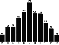 With two dice, numbers in the middle of the possible range come up more frequently, as there are more ways of getting them. Six different dice combinations give a result of 7 (what are they?), but only one combination will give a result of 2. So 7 is a more likely result than 2. Since each combination of dice is equally likely, the probability of getting a 7 is six times that of getting a 2.